
Methods
A multitask tool
Open science
French cities / regions
- Albi region
- Alençon St-Lô region
- Amiens region
- Angers region
- Angoulême region
- Annecy region
- Annemasse region
- Bayonne region
- Besançon region
- Béziers region
- Bordeaux region
- Brest region
- Caen region
- Carcassonne region
- Cherbourg region
- Clermont-Ferrand region
- Creil region
- Dijon region
- Douai region
- Dunkerque region
- Grenoble region
- La Réunion
- La Rochelle region
- Le Havre region
- Lille region
- Longwy region
Canadian cities / regions
Latin american cities / regions
Help to use the Mobiliscope
1) Preliminary notes
Initial data come from Origin-Destination surveys (from 2009 to 2019). Once transformed, these data have been used to estimate the ambient population in every district at exact hours (04.00, 05.00 etc.) during a typical weekday (Monday-Friday).
Number and proportion of ambient population aggregated by district and hour are estimation : they are subject to statistical margins of error.
58 city regions (spread over 5 countries) are included in the actual version of the Mobiliscope (v4.2).
To choose the city region you want to observe, please selection the city region in the drop-down menu ![]() or use the magnify tool
or use the magnify tool  from a search by name.
2) Select a map
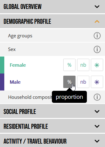
In the left-hand menu, you can choose indicator (classified into broad families such as demographic or social profile) and its map representation - eitheir as aof the total population, or number or flows.
To get informations about indicators, click button on the right side.
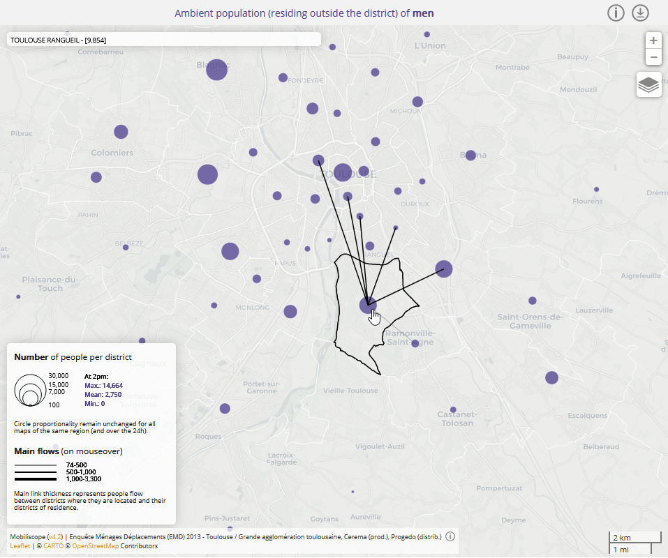
With flows maps you get number of non-resident people at district level. With links (displayed on mouseover), you can see their district of residence (not available on touch screens).
3) Change hours
At the top of the screen, click play button in the timeline to animate map and graphics according to the 24 hours of the day.

4) Explore a specific district
Select one district by clicking on the map.

Have a look at the chart entitled "In the selected district" where you can follow hourly variations of ambient population (for each group of the selected indicator) in the district under consideration. Colours have the same colour code than in the indicator menu. Here, last transportation mode used by present population in the selected district was coloured in blue for public transportation, in pink for private motor vehicle and in green for soft mobility.

By clicking on 'Unique' mode, you can limit representation of the hourly variations for only one subgroup :

5) Explore spatial segregation
The block of graphs entitled "In the whole region" displays two segregation indices computed from every district of the region for each hour of the day.
Duncan Index (also called Dissimilarity Index) measures the evenness with which a specific population subgroup is distributed across districts in a whole region. This index score can be interpreted as the percentage of people belonging to the subgroup under consideration that would have to move to achieve an even distribution in the whole region.
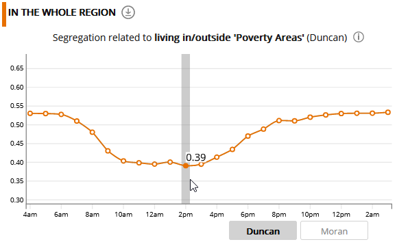
The example above displays, hour by hour, the Duncan Index (Paris region - 2010) for to ambient population residing in or outside 'Poverty Areas'. Duncan index range from 0 to 1. A Duncan Segregation Index value of 0 occurs when the share of ambient population residing in 'Poverty Areas' in every district is the same as the share of people residing in 'Poverty Areas' in the whole region. Conversely, a Duncan Segregation Index value of 1 occurs when each district gathers only one of the two population subgroups. In our example, Duncan value is found to be higher between 8pm and 7am, indicating a stronger segregation at night (further away from an even distribution): this corresponds to the hours when most of the individuals are at home or in their district of residence. The value of the index decreases during the day: because of their mobility, people residing in and outside of 'Poverty Areas' are more mixed (situation closer to even distribution).
By clicking on the "Moran" button, a second graph is displayed with the Moran index which measures the similarity in the profiles of the ambient population for neighbouring districts.

The Moran index values vary from -1 to +1: the closer its value is to 1, the more similar the spatially close districts are (with same distribution of the subgroup under consideration); the closer its value is to -1, the more dissimilar the spatially close districts are (with different distribution of the subgroup under consideration). When the Moran index value is 0, no similarity/dissimilarity pattern between neighbouring districts appears in the whole region. In our example, the Moran index values are positive and increase during the day: it means that spatial blocks of similar districts (according to the proportion of inhabitants of 'Poverty Areas') are formed during the day. This result does not contradict Duncan's index but complements it: people residing in 'Poverty Areas' visit during the day other districts than their residential district but tend to visit districts close to each other. And the same is true for people residing outside 'Poverty Areas'
It should be noted that in the case of an indicator subdivided into two groups (eg. male/female or people residing in/outside 'Poverty Areas'), Duncan and Moran values are the same for the two groups and therefore the curves are overlapping.
For more information on the two indices used (Duncan et Moran), click help button next to the index name.
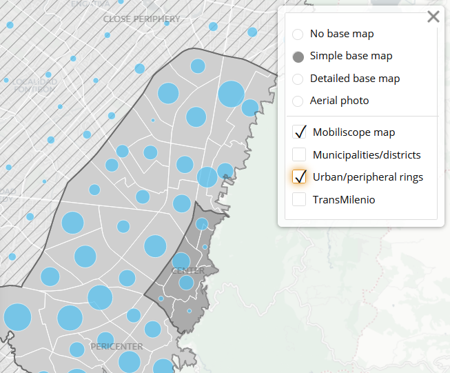
6) Change map backgrounds
By clicking on the  button in the central map, several layers can be displayed to make it easier to find your way around the interactive map: a simple base map (default layer), a more detailed one and aerial photos.


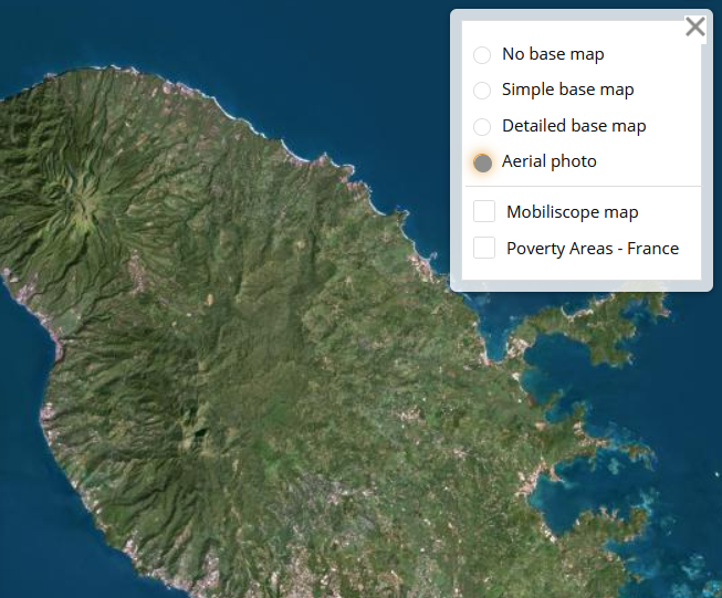
According to the city region under consideration, some other layers can also be displayed such as 'Poverty Areas' in French cities or urban/peripheral rings in Latin American cities.

7) Download data
Data displayed in the Mobiliscope are under open license (ODbL). Mobiliscope data are reusable as they remain under open license and that the sources are mentioned.
By clicking on the  button above the central map, you can download data aggregated data by district and by hour. By clicking on the button in the bottom graph, you can also download data about hourly segregation values (Duncan's or Moran's index) computed for the whole region over the 24 hours period.
To go further
To get more information about indicators and data which are currently used and displayed in the Mobiliscope, you can read Data, Indicators or Geovizualisation pages.
Enjoy!
Data
There are 58 city regions (in France, Canada and Latin America) included in the actual version of the Mobiliscope.
Origin-destination surveys
The data comes from large 'Origin-Destination' surveys
- French surveys are commissioned by local authorities, every 10 years or so, and carried out according to a standardised methodology developed by the Cerema (except for the Ile-de-France and its Global Transport Survey ; DRIEA-STIF-OMNIL). The majority of the surveys are available for research purposes through Progedo (National Archive of Data from Official Statistics in France). The remaining surveys come from the 'Unified Database' built by the Cerema and including all the French Origin-Destination surveys carried out since 2009. Some surveys are also available in open data (Nantes, Montpellier and Lille).
- Canadian surveys are provided by the Ministry of Transportation, Quebec.
- For Latin American cities, surveys are provided by: for Bogotá, the Sistema Integrado de información sobre Movilidad Urbana Regional (SIMUR); for Santiago, the Ministerio de Transportes y Telecomunicaciones, Programa de Vialidad y Transporte Urbano: SECTRA; for São Paulo, the Companhia do Metrô de São Paulo.
In the 'Origin-Destination' surveys, every trip made on the day before the survey was reported by respondents. The following variables were available for each trip: precise localisation of place of departure and place of arrival, time of departure and time of arrival (with exact minutes), trip purpose, and mode of transportation used. In the Canadian surveys, time of arrival was not requested from every respondent. These missing values have been replaced either from trip duration of comparable trips or from GIS computation.
Hourly district location
The Mobiliscope team has transformed the trip dataset into location dataset:
- 24 hourly time steps were defined to get 24 cross-sectional pictures of respondents' locations at exact hours (04.00, 05.00 etc.). Short locations in the interval between two exact hours are then not registered in district hourly dataset.
- Only trips occurring during the week (Monday-Friday) are considered to estimate hourly location during a typical weekday
- Transportation periods were also not considered except if respondents reported to use an 'adherent' mode of transportation (i.e. walking or cycling). In this case, half of the trip was considered as located in the district of origin and the other half as located in the district of destination. In the (rares) cases where 'adherent' trip symmetrically straddling an exact hour, location at this very hour was chosen to be in the district where respondent stayed the shortest time (because the longest duration taking place in the other district has a high probability to be registered at another hour).
Hourly location (which do not allow the re-identification of respondents) are displayed in the Mobiliscope. For French cities, theses hourly location data are freely downloadable and reusable, as they remain under open license (ODbL) and the sources are mentioned. Data can be downloaded by clicking the button above the central map.
Studied population
Only respondents aged 16 years and over (or aged 15 years and over in Canadian cities) are taken into consideration.
Measures displayed in the Mobiliscope have been estimated taking into account weighting coefficients to grant the same distribution and the same population size than observed in population census.
- In French cities, weighting coefficients are based on household profile (size and housing type) and on individual profile (age, sex, and for the Paris Region, occupation and socioprofessional group).
- In Canadian cities, weighting coefficients are only based on sex and age of participants.
- In Bogotá, weighting coefficients were adjusted on the number of households enumerated by the census. In Santiago, weighting coefficients are based on household profile (size and vehicle equipment) and on individual profile (age, sex). In São Paulo, we do not have all the elements.
Districts
In the Mobiliscope, cities have been subdivided into districts. Districts are smaller in inner cities and larger in the peripheral areas. In every city region, there is roughly the same number of surveyed residents by district. District was the smallest unit in which it is relevant to aggregate data when it comes to not only ensuring sufficient sample size for statistical analysis but also protecting confidentiality of personal data for the provision of open data.
- In French cities, districts (called 'secteurs' in French 'Origin-Destination' surveys) are the primary sampling units. They correspond to large neighbourhoods in urban areas and to a 'commune' (or a group of communes) in suburban/peripheral areas. When more than three communes are included in one district, only the names of the three more populated are displayed on mouseover.
- In Canadian cities, districts correspond to municipalities.
- In Bogotá, districts correspond to the primary sampling units (named UTAM). Nevertheless, the map backgrounds used in the Mobiliscope are those reworked by Florent Demoraes as part of the ANR MODURAL project, allowing the large, very sparsely populated sectors to be readjusted to the contours of the areas actually inhabited and surveyed.
- In Santiago, districts were defined by the Mobiliscope team based on the spatial units defined by the Origin-Destination survey, the zonas, according to an objective in terms of the minimum number of residents surveyed aged 16 and over (at least 100) and by preserving as much as possible the coherence of the administrative divisions and their social composition.
- For São Paulo, districts were also defined by the Mobiliscope team and correspond to the Distritos within the municipio of São Paulo and, outside the municipio, to the zonas defined by the Origin-Destination survey.
More methodological details can be found in the paper Social segregation around the clock in the Paris region (France).
Survey description for every city region
Respondents aged 15 yrs. and over in Canada or aged 16 yrs. and over in the other cities
| City region | Year | Number of respondents | Number of weekdays trips | Number of hourly locations | Number of districts | District size in km². Median area (min-max) | Number of respondents per district. Median (min-max) at 3am | Number of respondents per district. Median (min-max) at 3pm |
|---|---|---|---|---|---|---|---|---|
| Albi region | 2011 | 2,339 | 9,171 | 52,709 | 15 | 7 (1.3-54) | 155 (148-160) | 119 (77-288) |
| Alençon region | 2018 | 6,520 | 30,315 | 148,702 | 46 | 145 (1.9-435) | 140 (131-154) | 118 (78-231) |
| Amiens region | 2010 | 7,097 | 30,933 | 162,293 | 45 | 13 (0.8-410) | 145 (127-238) | 128 (76-443) |
| Angers region | 2012 | 3,983 | 18,399 | 90,032 | 28 | 17 (2-111) | 138 (124-160) | 111 (63-258) |
| Angoulême region | 2012 | 2,684 | 11,300 | 60,691 | 18 | 14 (1.5-151) | 146 (139-172) | 130 (75-249) |
| Annecy region | 2017 | 4,953 | 22,944 | 110,641 | 34 | 27 (0.9-486) | 143 (130-172) | 124 (83-246) |
| Annemasse region | 2016 | 5,905 | 26,700 | 123,973 | 42 | 36 (0.8-232) | 137 (121-213) | 96 (66-161) |
| Bayonne region | 2010 | 7,387 | 28,716 | 170,184 | 50 | 20 (0.8-642) | 147 (129-171) | 122 (86-436) |
| Besançon region | 2018 | 3,980 | 17,568 | 90,654 | 28 | 5 (0.5-191) | 142 (127-157) | 104 (74-451) |
| Béziers region | 2014 | 4,212 | 18,661 | 95,887 | 30 | 52 (1.2-822) | 138 (130-153) | 117 (82-204) |
| Bogotá region | 2019 | 49,757 | 127,405 | 1,126,901 | 133 | 4 (0.8-15) | 365 (46-729) | 323 (70-1453) |
| Bordeaux region | 2009 | 13,793 | 60,641 | 321,385 | 95 | 10 (0.4-1206) | 142 (124-216) | 127 (61-293) |
| Brest region | 2018 | 6,518 | 29,237 | 151,004 | 46 | 13 (0.9-236) | 139 (125-161) | 115 (73-301) |
| Caen region | 2011 | 10,000 | 43,194 | 232,512 | 67 | 15 (0.5-647) | 151 (125-165) | 123 (70-485) |
| Carcassonne region | 2015 | 2,891 | 11,915 | 66,165 | 19 | 36 (0.8-246) | 153 (140-159) | 119 (90-306) |
| Cherbourg region | 2016 | 4,207 | 18,978 | 97,670 | 28 | 42 (1.3-231) | 150 (142-158) | 125 (88-337) |
| Clermont-Ferrand region | 2012 | 8,052 | 34,182 | 187,334 | 56 | 39 (0.7-471) | 144 (130-159) | 112 (71-373) |
| Creil region | 2017 | 4,581 | 18,956 | 96,753 | 31 | 16 (1-144) | 146 (140-153) | 104 (60-199) |
| Dijon region | 2016 | 4,372 | 18,685 | 100,771 | 30 | 6 (0.7-241) | 142 (126-179) | 120 (67-341) |
| Douai region | 2012 | 5,344 | 23,883 | 115,844 | 38 | 8 (1-54) | 139 (127-160) | 110 (64-214) |
| Dunkerque region | 2015 | 4,537 | 22,491 | 103,897 | 32 | 9 (1.1-117) | 140 (128-154) | 114 (71-289) |
| Grenoble region | 2010 | 13,834 | 63,336 | 318,862 | 97 | 14 (0.2-834) | 139 (124-273) | 107 (50-471) |
| La Réunion region | 2016 | 13,801 | 53,363 | 324,660 | 99 | 11 (0.6-275) | 139 (121-159) | 124 (72-317) |
| La Rochelle region | 2011 | 2,902 | 12,203 | 66,249 | 19 | 8 (1.3-40) | 153 (137-164) | 120 (75-401) |
| Le Havre region | 2018 | 6,540 | 29,029 | 151,581 | 43 | 25 (0.7-256) | 141 (127-262) | 108 (72-434) |
| Lille region | 2016 | 7,949 | 38,180 | 181,210 | 57 | 5 (1-56) | 138 (123-156) | 118 (76-323) |
| Longwy region | 2014 | 3,347 | 13,178 | 70,548 | 22 | 32 (2.2-200) | 152 (145-160) | 108 (79-155) |
| Lyon region | 2015 | 24,070 | 99,585 | 557,575 | 169 | 10 (0.4-346) | 140 (121-251) | 122 (68-445) |
| Marseille region | 2009 | 19,380 | 87,031 | 449,111 | 137 | 18 (0.3-342) | 141 (117-165) | 118 (66-401) |
| Martinique region | 2014 | 4,179 | 14,005 | 98,073 | 24 | 36 (4.7-129) | 156 (129-283) | 146 (110-296) |
| Metz region | 2017 | 6,490 | 31,131 | 144,399 | 44 | 13 (1.1-176) | 142 (129-238) | 112 (70-414) |
| Montpellier region | 2014 | 11,433 | 52,387 | 263,639 | 80 | 10 (0.3-547) | 140 (126-236) | 114 (71-421) |
| Montréal region | 2013 | 155,853 | 404,563 | 3,689,524 | 113 | 36 (1-762) | 1069 (116-4551) | 862 (109-9656) |
| Nancy region | 2013 | 9,657 | 40,664 | 221,489 | 68 | 17 (0.6-407) | 142 (124-163) | 110 (57-542) |
| Nantes region | 2015 | 17,357 | 81,924 | 401,110 | 123 | 21 (0.6-331) | 138 (113-195) | 117 (66-389) |
| Nice region | 2009 | 14,989 | 58,239 | 346,893 | 104 | 5 (0.4-505) | 143 (128-163) | 126 (65-384) |
| Nîmes region | 2015 | 4,519 | 18,598 | 102,599 | 31 | 8 (0.3-152) | 144 (132-168) | 114 (75-327) |
| Niort region | 2016 | 2,869 | 12,705 | 65,026 | 19 | 15 (1.1-156) | 150 (142-160) | 130 (83-226) |
| Ottawa-Gatineau region | 2011 | 48,767 | 149,147 | 1,159,530 | 26 | 58 (2.6-1278) | 1792 (400-4367) | 1566 (338-4695) |
| Paris region | 2010 | 26,312 | 124,258 | 605,074 | 109 | 26 (3-1324) | 235 (129-420) | 204 (86-746) |
| Poitiers region | 2018 | 4,106 | 17,305 | 93,297 | 28 | 51 (1.1-228) | 140 (127-255) | 104 (60-450) |
| Québec region | 2011 | 48,660 | 135,788 | 1,128,494 | 69 | 16 (1.5-697) | 666 (301-1553) | 527 (179-2415) |
| Quimper region | 2013 | 4,696 | 17,291 | 108,273 | 30 | 57 (2.5-260) | 152 (142-200) | 130 (96-285) |
| Rennes region | 2018 | 9,317 | 44,004 | 214,867 | 68 | 55 (0.8-466) | 136 (118-159) | 106 (64-379) |
| Rouen region | 2017 | 8,905 | 38,146 | 202,329 | 63 | 15 (1.1-231) | 140 (118-166) | 108 (59-295) |
| Saguenay region | 2015 | 13,942 | 41,229 | 327,391 | 21 | 26 (3.2-616) | 667 (456-760) | 601 (326-1200) |
| Saint-Brieuc region | 2012 | 3,570 | 14,556 | 80,240 | 22 | 8 (1.1-35) | 152 (146-245) | 124 (71-377) |
| Saint-Étienne region | 2010 | 8,525 | 38,576 | 195,223 | 52 | 30 (1.2-345) | 156 (137-220) | 127 (78-331) |
| Santiago region | 2012 | 29,733 | 75,733 | 685,001 | 185 | 3 (0.7-855) | 156 (93-412) | 121 (58-1130) |
| São Paulo region | 2017 | 71,866 | 152,975 | 1,690,002 | 259 | 11 (1.3-522) | 146 (60-1540) | 162 (40-1870) |
| Sherbrooke region | 2012 | 19,908 | 58,361 | 456,828 | 28 | 22 (1.7-357) | 668 (533-1245) | 504 (329-1517) |
| Strasbourg region | 2009 | 10,052 | 46,935 | 231,463 | 67 | 35 (0.6-581) | 145 (128-225) | 123 (78-284) |
| Thionville region | 2012 | 3,609 | 15,676 | 75,299 | 22 | 7 (0.6-62) | 164 (155-173) | 106 (80-243) |
| Toulouse region | 2013 | 11,141 | 48,919 | 257,168 | 66 | 11 (0.9-237) | 154 (128-331) | 128 (64-530) |
| Tours region | 2019 | 7,624 | 33,388 | 175,782 | 54 | 43 (0.5-637) | 139 (122-160) | 119 (78-279) |
| Trois-Rivières region | 2011 | 18,936 | 50,687 | 433,505 | 28 | 62 (1.9-305) | 562 (422-1514) | 427 (284-1443) |
| Valence region | 2014 | 5,143 | 23,230 | 117,368 | 36 | 41 (1.3-477) | 142 (127-163) | 122 (71-326) |
| Valenciennes region | 2019 | 5,647 | 46,441 | 126,662 | 41 | 12 (0.9-51) | 137 (125-150) | 112 (75-255) |
