
Methods
A multitask tool
Open science
French cities / regions
- Albi region
- Alençon St-Lô region
- Amiens region
- Angers region
- Angoulême region
- Annecy region
- Annemasse region
- Bayonne region
- Besançon region
- Béziers region
- Bordeaux region
- Brest region
- Caen region
- Carcassonne region
- Cherbourg region
- Clermont-Ferrand region
- Creil region
- Dijon region
- Douai region
- Dunkerque region
- Grenoble region
- La Réunion
- La Rochelle region
- Le Havre region
- Lille region
- Longwy region
Canadian cities / regions
Latin american cities / regions
Help to use the Mobiliscope
1) Preliminary notes
Initial data come from Origin-Destination surveys (from 2009 to 2019). Once transformed, these data have been used to estimate the ambient population in every district at exact hours (04.00, 05.00 etc.) during a typical weekday (Monday-Friday).
Number and proportion of ambient population aggregated by district and hour are estimation : they are subject to statistical margins of error.
58 city regions (spread over 5 countries) are included in the actual version of the Mobiliscope (v4.2).
To choose the city region you want to observe, please selection the city region in the drop-down menu ![]() or use the magnify tool
or use the magnify tool  from a search by name.
2) Select a map
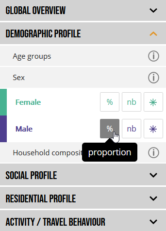
In the left-hand menu, you can choose indicator (classified into broad families such as demographic or social profile) and its map representation - eitheir as aof the total population, or number or flows.
To get informations about indicators, click button on the right side.
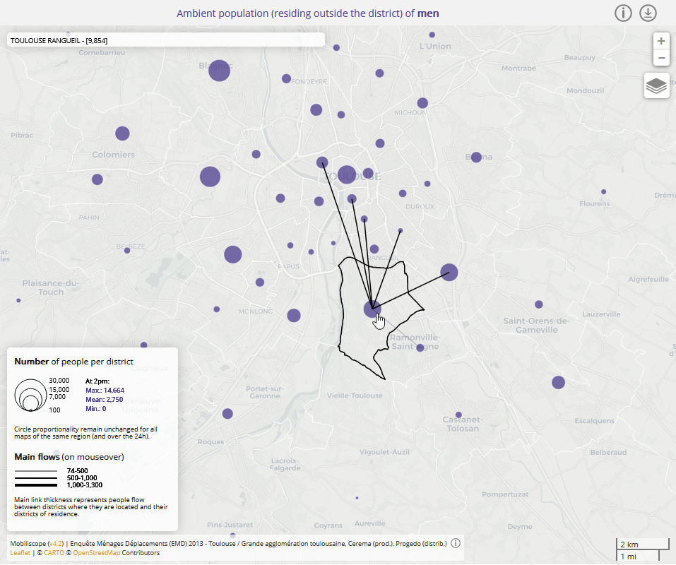
With flows maps you get number of non-resident people at district level. With links (displayed on mouseover), you can see their district of residence (not available on touch screens).
3) Change hours
At the top of the screen, click play button in the timeline to animate map and graphics according to the 24 hours of the day.

4) Explore a specific district
Select one district by clicking on the map.

Have a look at the chart entitled "In the selected district" where you can follow hourly variations of ambient population (for each group of the selected indicator) in the district under consideration. Colours have the same colour code than in the indicator menu. Here, last transportation mode used by present population in the selected district was coloured in blue for public transportation, in pink for private motor vehicle and in green for soft mobility.

By clicking on 'Unique' mode, you can limit representation of the hourly variations for only one subgroup :

5) Explore spatial segregation
The block of graphs entitled "In the whole region" displays two segregation indices computed from every district of the region for each hour of the day.
Duncan Index (also called Dissimilarity Index) measures the evenness with which a specific population subgroup is distributed across districts in a whole region. This index score can be interpreted as the percentage of people belonging to the subgroup under consideration that would have to move to achieve an even distribution in the whole region.
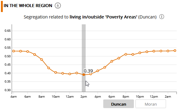
The example above displays, hour by hour, the Duncan Index (Paris region - 2010) for to ambient population residing in or outside 'Poverty Areas'. Duncan index range from 0 to 1. A Duncan Segregation Index value of 0 occurs when the share of ambient population residing in 'Poverty Areas' in every district is the same as the share of people residing in 'Poverty Areas' in the whole region. Conversely, a Duncan Segregation Index value of 1 occurs when each district gathers only one of the two population subgroups. In our example, Duncan value is found to be higher between 8pm and 7am, indicating a stronger segregation at night (further away from an even distribution): this corresponds to the hours when most of the individuals are at home or in their district of residence. The value of the index decreases during the day: because of their mobility, people residing in and outside of 'Poverty Areas' are more mixed (situation closer to even distribution).
By clicking on the "Moran" button, a second graph is displayed with the Moran index which measures the similarity in the profiles of the ambient population for neighbouring districts.

The Moran index values vary from -1 to +1: the closer its value is to 1, the more similar the spatially close districts are (with same distribution of the subgroup under consideration); the closer its value is to -1, the more dissimilar the spatially close districts are (with different distribution of the subgroup under consideration). When the Moran index value is 0, no similarity/dissimilarity pattern between neighbouring districts appears in the whole region. In our example, the Moran index values are positive and increase during the day: it means that spatial blocks of similar districts (according to the proportion of inhabitants of 'Poverty Areas') are formed during the day. This result does not contradict Duncan's index but complements it: people residing in 'Poverty Areas' visit during the day other districts than their residential district but tend to visit districts close to each other. And the same is true for people residing outside 'Poverty Areas'
It should be noted that in the case of an indicator subdivided into two groups (eg. male/female or people residing in/outside 'Poverty Areas'), Duncan and Moran values are the same for the two groups and therefore the curves are overlapping.
For more information on the two indices used (Duncan et Moran), click help button next to the index name.
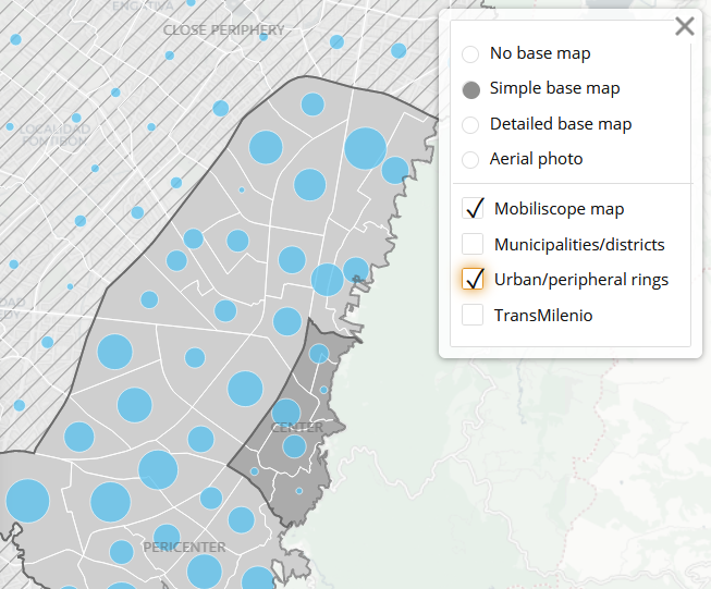
6) Change map backgrounds
By clicking on the  button in the central map, several layers can be displayed to make it easier to find your way around the interactive map: a simple base map (default layer), a more detailed one and aerial photos.


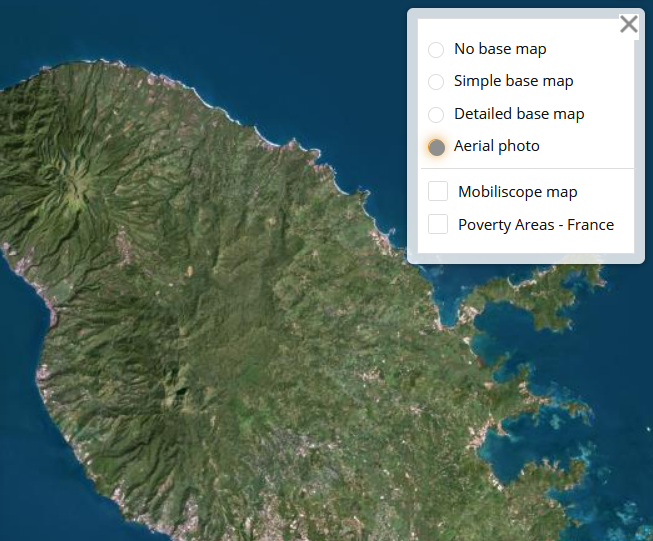
According to the city region under consideration, some other layers can also be displayed such as 'Poverty Areas' in French cities or urban/peripheral rings in Latin American cities.

7) Download data
Data displayed in the Mobiliscope are under open license (ODbL). Mobiliscope data are reusable as they remain under open license and that the sources are mentioned.
By clicking on the  button above the central map, you can download data aggregated data by district and by hour. By clicking on the button in the bottom graph, you can also download data about hourly segregation values (Duncan's or Moran's index) computed for the whole region over the 24 hours period.
To go further
To get more information about indicators and data which are currently used and displayed in the Mobiliscope, you can read Data, Indicators or Geovizualisation pages.
Enjoy!
Indicators
In the Mobiliscope, people can be characterised according to their demographic and social profile and their residential area, as well as the nature of their activity and the last mode of travel they used to reach their destination.
Global overview
- Whole population. It displays the whole ambient population (aged 16 years and over; for Canadian cities aged 15 and over).
- Residing in/out the district. The whole ambient population has been divided into two groups (residing in the district versus residing outside the district)
Demographic profile
- Age divided into four groups: 16-24 years (15-24 for Canadian cities); 25-34 years; 35-64 years; 65 and more.
- Sex: Female and Male.
- Household composition This indicator defines the household type in which people live:
- For French cities, household composition is categorised into four groups: single person; couple without children (referent person of the household or his/her partner); household (excluding couple) without children (i.e. members of a household composed only of adults, without children under 16); household with children (i.e. members of a household composed of one or more adults with child(ren) under 16 - members are not necessarily related to each other).
- For Canadian cities, household composition is categorised into three groups: single person; household without children (i.e. members of a household composed of adults only, with no children under 15); household with children (i.e. members of a household composed of one or more adults with child(ren) under 15 - members are not necessarily related to each other).
- For Latin American cities, household composition is categorised into five groups: single person; nuclear family without children (i.e. members with direct filial relationship without children under 16); complex household without children (i.e. at least one member without a direct filial relationship and without child under 16); nuclear family with children (i.e. members with a direct filial relationship with at least one child under 16); complex household with children (i.e. at least one member without a direct filial relationship and with at least one child under 16).
Social profile
Indicators relative to the social profile are different from one city to another.
In French cities
- Educational level . We merged respondent's achieved level of education in four groups of individual educational status: low (middle school or less); middle-low (high school without Baccalauréat); middle-high (up to two years after Baccalauréat); and high (three years or more after Baccalauréat).
We also computed household educational status corresponding to the lowest level of education of the adults in the household. - Socioprofessional status. We merged socioprofessional data in five groups of individual socioprofessional status: inactive (unemployed long term, housework); workers; employees; intermediate occupations (intermediary professionals, craftsmen, merchants, employers of more than 10 employees and farm operators); and managers and higher intellectual professionals. We also computed household socioprofessional status corresponding to the lowest socioprofessional category of the adults in the household.
- Occupational status in five groups: inactive; retired; unemployed; student; active.
- Household income - only for the Paris region. Monthly household income has been divided by the number of adults and children in the household to get household income per consumption units (CU). We distinguished four groups: low (< 1,084€/CU); middle-low (1,084-1,806€/CU); middle-high (1,806-2,890€/CU); high (>2,890€/CU). Income intervals have been defined according to median household income in the Paris region (equal to 1,806€/CU in 2010). The first threshold (1,084€/CU) or 'poverty threshold' corresponds to 60% of median household income; the second one (1806€/CU) corresponds to the median household income; the third one (2,890€/CU) corresponds to 160% of median household income.
In Canadian cities
- Household income. Annual household income (after tax) has been divided by the number of adults and children in the household. We distinguished four groups: low (< 19,669$/year); middle-low (19,669-39,337$/year); middle-high (39337-68840$/year); high (>68,840$/year). Income intervals have been defined according to median household income for a one-person household in Quebec (equal to 39337$/year in 2015). The first threshold (19669$/year) or 'low income measure' corresponds to 50% of median household income; the second one (39,337$/year) corresponds to the median household income; the third one (68,840$/year) corresponds to 175% of median household income. Because of large number of missing incomes (20%), an additional 'missing' class has been added
- Occupational status in five groups: inactive; retired; unemployed; student; active.
In Latin American cities
- Level of education based on the last degree obtained by the respondents. We aggregated individual education levels into four groups: low (less than 9 years of studies); intermediate (between 9 and 11 years of studies); high (between 12 and 15 years of studies); and very high (at least 16 years of studies). Education level was also measured at the household level based on the highest level of education of adults in the household.
- Household income. Income has been divided by the number of adults and children in the household. We distinguished five groups: very low; low; intermediate; high; very high. The ranges chosen for each city were defined according to the national minimum salary. Imputation methods were used for missing data.
- Socioprofessional status. The active population was divided into four categories: unskilled workers; skilled workers; self-employed ; and executives and higher intellectual professions.
- Occupational status into five groups: inactive; retired; unemployed; student; active.
- Professional informality for Bogotá and São Paulo only. Informal work was approached by combining the category of employment and the economic sector of the employing firm, following the methods proposed by the International Labor Organization (ILO). When information was insufficient to follow the decision rules advocated by the ILO, education and income level have also been used.
Residential area
Indicators about the profile of residential areas are available in French and Latine America cities.
In French cities
- Residential location in the urban/peripheral rings. Three areas were defined: inner city ; urban area ; suburban/peripheral area. 'Inner city' refers to central (administrative) city in charge of the origin-destination survey. 'Urban area' refers to districts which are totally (or mainly) included in large, middle or small urban clusters as defined in the 2010 'Zoning into Urban Areas - ZAU' (French National Institute of Statistics and Economic Studies). The remaining districts have been labelled as belonging to 'suburban/peripheral area'.
- Residential location in/outside 'Poverty Areas' (Quartiers Prioritaires en Politique de la Ville - QPV ). Respondents have been divided into two groups (living in or outside 'Poverty Areas') according to the overlap between their local area of residence (called 'zone fine' in the French survey) and the boundaries of the 'Poverty Areas' (Quartiers prioritaires de la Politique de la Ville - QPV). Since French Origin-Destination surveys do not provide information on the exact residential location, respondents have been defined as living in 'Poverty Areas' if their local areas of residence include a majority (> 51%) of population in 'Poverty Areas' according to 2013 population census. Note that there are 'Priority Areas' in every French city region in the Mobiliscope except for the Annecy region.
- Departments of residence- only for the Paris region.
In Latin American cities
- Residential location in the urban/peripheral rings. Rings were divided into 4 groups: center; pericenter; close periphery; distant periphery. This division is based on the one proposed in the book Mobilities and Urban Change. Bogotá, Santiago and São Paulo edited by F. Dureau, T. Lulle, S. Souchaud and Y. Contreras (2014).
- Socio-economic stratum of residence - for Bogotá only. Socioeconomic stratification is a typology of Colombian public actors to establish the rates of public services available for households according to their place of residence: dwellings were described according to the characteristics of the dwellings and their close environment (quality of the building, roadway, presence of facilities, etc).
- Housing tenure. We consider the status of the household dwelling (ownership, rental, usufruct, etc.) and the place of the respondent in the household and define three tenure status: owner (when the person - or his/her partner - owns the dwelling); tenant (when the person - or his/her partner - rents the dwelling); rent-free tenants (when the person lives - or his/her partner - in a dwelling without owning or renting it). Usufructuaries, persons occupying a dwelling free of charge or housed in an owner-occupied or tenant-occupied dwelling are included in this category. For respondents under 25 living with their parents, the tenure status of the parents is considered.
Activity/Travel behaviour
In contrast with indicators related to individual/household characteristics, indicators related to activity and travel mode may change for one individual throughout the day.
- Activity places. From trip purposes, we isolated activities performed at home and we distinguished 4 activities performed in out-of-home places: working, studying, shopping, leisure (recreational, cultural or sporting activities, family and personal visits). For French and Canadian cities, we have excluded 'unspecified activity' and 'activity related to chaperoning or chauffeuring'. The sample of locations related to these activities was too small and it does not make sense to gather them with some other activities. For Latin American cities only, we introduced another category to group together administrative and so-called "personal" activities (including accompanying activities) motivating a significant proportion of trips.
- Last travel mode. It concerns the last travel mode used to reach destination. Three groups modes have been distinguished: soft mobility (walking, cycling...), individual motor vehicle (two-wheeled motor vehicle, personal cars or motorcycles, cabs...) and collective transportation (bus, metro, train, tram, company transport...). For Bogotá, the TransMilenio and its network of secondary buses were isolated from collective transportation as a separate group. If more than one mode of transport is used during a trip (so-called 'multi-modal' trips), the main mode is established by giving priority to collective transport, then to individual motor vehicle and finally to soft mobility. Thus, a trip in which bus and private car has been used is classified as a trip made mainly by collective transportation.
Detailed informations about indicators sample size for every city region
Respondents aged 15 yrs. and over in Canada or aged 16 yrs. and over in the other cities
| City region | Year | Number of respondents | With socioprof. status at household/indiv.level | With education data at household/indiv. level | With household income | With occupational status | With activity at 6pm/at 3am | With travel mode at 6pm/at 3am |
|---|---|---|---|---|---|---|---|---|
| Albi region | 2011 | 2,339 | 2,292/ 2,205 | 2,292/ 2,205 | - | 2,298 | 2,130/ 2,325 | 1,802/ 1,998 |
| Alençon region | 2018 | 6,520 | 6,443/ 6,313 | 6,443/ 6,313 | - | 6,399 | 6,003/ 6,489 | 5,168/ 5,662 |
| Amiens region | 2010 | 7,097 | 6,773/ 6,384 | 6,768/ 6,364 | - | 7,054 | 6,560/ 7,066 | 5,609/ 6,127 |
| Angers region | 2012 | 3,983 | 3,840/ 3,611 | 3,844/ 3,617 | - | 3,917 | 3,597/ 3,965 | 3,187/ 3,569 |
| Angoulême region | 2012 | 2,684 | 2,617/ 2,489 | 2,617/ 2,489 | - | 2,635 | 2,442/ 2,673 | 2,145/ 2,380 |
| Annecy region | 2017 | 4,953 | 4,885/ 4,712 | 4,889/ 4,717 | - | 4,901 | 4,428/ 4,917 | 3,823/ 4,327 |
| Annemasse region | 2016 | 5,905 | 5,830/ 5,590 | 5,838/ 5,603 | - | 5,833 | 4,935/ 5,871 | 4,386/ 5,328 |
| Bayonne region | 2010 | 7,387 | 7,328/ 6,944 | 6,874/ 6,395 | - | 7,246 | 6,858/ 7,374 | 5,691/ 6,215 |
| Besançon region | 2018 | 3,980 | 3,776/ 3,590 | 3,777/ 3,591 | - | 3,947 | 3,657/ 3,965 | 3,222/ 3,537 |
| Béziers region | 2014 | 4,212 | 4,154/ 4,068 | 4,140/ 4,047 | - | 4,011 | 3,910/ 4,204 | 3,371/ 3,672 |
| Bogotá region | 2019 | 49,757 | -/26,762 | 49,750/49,756 | 49,757 | 48,038 | 44,986/ 49,482 | 36,012/ 40,688 |
| Bordeaux region | 2009 | 13,793 | 13,349/12,465 | 12,510/11,557 | - | 13,596 | 12,899/ 13,770 | 11,267/ 12,156 |
| Brest region | 2018 | 6,518 | 6,313/ 6,050 | 6,313/ 6,050 | - | 6,352 | 6,114/ 6,502 | 5,443/ 5,841 |
| Caen region | 2011 | 10,000 | 9,674/ 9,134 | 8,706/ 8,126 | - | 9,778 | 9,443/ 9,982 | 8,195/ 8,747 |
| Carcassonne region | 2015 | 2,891 | 2,843/ 2,781 | 2,843/ 2,781 | - | 2,854 | 2,705/ 2,883 | 2,267/ 2,447 |
| Cherbourg region | 2016 | 4,207 | 4,144/ 4,021 | 4,144/ 4,021 | - | 4,136 | 3,970/ 4,198 | 3,377/ 3,609 |
| Clermont-Ferrand region | 2012 | 8,052 | 7,776/ 7,387 | 7,777/ 7,388 | - | 7,907 | 7,619/ 8,044 | 6,609/ 7,051 |
| Creil region | 2017 | 4,581 | 4,467/ 4,277 | 4,467/ 4,278 | - | 4,483 | 3,813/ 4,534 | 3,317/ 4,046 |
| Dijon region | 2016 | 4,372 | 4,172/ 3,887 | 4,173/ 3,901 | - | 4,321 | 4,102/ 4,355 | 3,616/ 3,872 |
| Douai region | 2012 | 5,344 | 5,324/ 4,921 | 5,322/ 4,928 | - | 5,230 | 4,677/ 5,300 | 3,807/ 4,439 |
| Dunkerque region | 2015 | 4,537 | 4,500/ 4,230 | 4,501/ 4,235 | - | 4,466 | 4,226/ 4,523 | 3,600/ 3,904 |
| Grenoble region | 2010 | 13,834 | 13,375/12,338 | 13,355/12,301 | - | 13,528 | 12,810/ 13,803 | 11,287/ 12,303 |
| La Réunion region | 2016 | 13,801 | 13,663/12,618 | 13,671/12,639 | 24,449 | 25,944 | 23,485/ 26,280 | 21,610/ 24,463 |
| La Rochelle region | 2011 | 2,902 | 2,831/ 2,712 | 2,832/ 2,713 | - | 13,557 | 13,312/ 13,801 | 10,398/ 10,904 |
| Le Havre region | 2018 | 6,540 | 6,434/ 6,150 | 6,434/ 6,150 | - | 2,817 | 2,663/ 2,894 | 2,344/ 2,577 |
| Lille region | 2016 | 7,949 | 7,458/ 6,797 | 7,436/ 6,752 | - | 6,440 | 6,150/ 6,523 | 5,202/ 5,587 |
| Longwy region | 2014 | 3,347 | 3,290/ 3,193 | 3,296/ 3,206 | - | 7,825 | 7,244/ 7,913 | 6,345/ 7,023 |
| Lyon region | 2015 | 24,070 | 22,981/21,433 | 22,986/21,445 | - | 3,287 | 2,907/ 3,322 | 2,350/ 2,771 |
| Marseille region | 2009 | 19,380 | 19,122/17,697 | 19,112/17,626 | - | 23,735 | 22,448/ 24,008 | 19,561/ 21,173 |
| Martinique region | 2014 | 4,179 | 4,163/ 3,849 | 4,164/ 3,855 | - | 18,975 | 18,116/ 19,339 | 15,812/ 17,072 |
| Metz region | 2017 | 6,490 | 6,321/ 5,969 | 6,319/ 5,962 | - | 4,109 | 4,044/ 4,178 | 2,903/ 3,041 |
| Montpellier region | 2014 | 11,433 | 10,644/ 9,946 | 10,650/ 9,960 | - | 6,423 | 5,801/ 6,447 | 5,022/ 5,681 |
| Montréal region | 2013 | 155,853 | -/- | -/- | - | 11,237 | 10,644/ 11,405 | 9,340/ 10,122 |
| Nancy region | 2013 | 9,657 | 9,100/ 8,511 | 9,110/ 8,520 | 155,853 | 155,790 | 152,262/155,762 | 119,949/124,042 |
| Nantes region | 2015 | 17,357 | 16,895/16,060 | 16,908/16,066 | - | 9,439 | 8,942/ 9,628 | 7,620/ 8,327 |
| Nice region | 2009 | 14,989 | 14,905/14,021 | 12,742/10,537 | - | 17,134 | 16,045/ 17,314 | 14,079/ 15,372 |
| Nîmes region | 2015 | 4,519 | 4,432/ 4,137 | 4,428/ 4,124 | - | 14,752 | 13,960/ 14,963 | 11,737/ 12,761 |
| Niort region | 2016 | 2,869 | 2,805/ 2,732 | 2,805/ 2,732 | - | 4,383 | 4,151/ 4,502 | 3,396/ 3,753 |
| Ottawa-Gatineau region | 2011 | 48,767 | -/- | -/- | - | 2,828 | 2,601/ 2,858 | 2,255/ 2,514 |
| Paris region | 2010 | 26,312 | 26,003/23,814 | 25,936/23,696 | 48,767 | 48,767 | 47,908/ 48,759 | 38,777/ 39,756 |
| Poitiers region | 2018 | 4,106 | 3,730/ 3,603 | 3,730/ 3,603 | - | 4,045 | 3,742/ 4,075 | 3,299/ 3,641 |
| Québec region | 2011 | 48,660 | -/- | -/- | 48,660 | 48,660 | 46,738/ 48,408 | 38,488/ 40,284 |
| Quimper region | 2013 | 4,696 | 4,639/ 4,519 | 4,639/ 4,519 | - | 4,550 | 4,384/ 4,680 | 3,626/ 3,925 |
| Rennes region | 2018 | 9,317 | 9,007/ 8,589 | 9,007/ 8,589 | - | 9,254 | 8,580/ 9,275 | 7,663/ 8,379 |
| Rouen region | 2017 | 8,905 | 8,568/ 7,930 | 8,580/ 7,952 | - | 8,746 | 8,064/ 8,872 | 6,896/ 7,722 |
| Saguenay region | 2015 | 13,942 | -/- | -/- | 13,942 | 13,942 | 13,668/ 13,904 | 10,449/ 10,719 |
| Saint-Brieuc region | 2012 | 3,570 | 3,517/ 3,403 | 3,517/ 3,403 | - | 3,503 | 3,219/ 3,543 | 2,840/ 3,168 |
| Saint-Étienne region | 2010 | 8,525 | 8,365/ 7,788 | 8,346/ 7,740 | - | 8,309 | 7,922/ 8,499 | 6,671/ 7,257 |
| Santiago region | 2012 | 29,733 | -/15,757 | 29,733/29,732 | 29,733 | 29,732 | 27,513/ 29,608 | 22,457/ 24,768 |
| São Paulo region | 2017 | 71,866 | -/41,190 | 71,858/71,866 | 71,866 | 71,866 | 67,909/ 71,844 | 45,292/ 49,373 |
| Sherbrooke region | 2012 | 19,908 | -/- | -/- | 19,908 | 19,908 | 19,017/ 19,718 | 15,109/ 15,850 |
| Strasbourg region | 2009 | 10,052 | 9,789/ 9,016 | 9,714/ 8,811 | - | 9,886 | 9,320/ 10,029 | 8,154/ 8,881 |
| Thionville region | 2012 | 3,609 | 3,516/ 3,318 | 3,515/ 3,317 | - | 3,551 | 3,020/ 3,582 | 2,549/ 3,113 |
| Toulouse region | 2013 | 11,141 | 9,992/ 9,207 | 10,011/ 9,216 | - | 11,032 | 10,234/ 11,115 | 9,055/ 9,953 |
| Tours region | 2019 | 7,624 | 7,336/ 7,040 | 7,336/ 7,040 | - | 7,530 | 7,069/ 7,589 | 6,070/ 6,603 |
| Trois-Rivières region | 2011 | 18,936 | -/- | -/- | 18,936 | 18,936 | 18,132/ 18,819 | 13,439/ 14,186 |
| Valence region | 2014 | 5,143 | 5,089/ 4,867 | 5,091/ 4,874 | - | 5,026 | 4,735/ 5,124 | 4,057/ 4,453 |
| Valenciennes region | 2019 | 5,647 | 5,515/ 5,214 | 5,515/ 5,214 | - | 5,517 | 5,150/ 5,616 | 4,249/ 4,730 |
